

BigQuery cost optimization refers to the process of minimizing unnecessary expenditures while still meeting the performance and data analysis requirements.
Contrary to popular belief, Google BigQuery is a cost-effective solution. However, it can get expensive pretty fast in the hands of a rookie.
BigQuery Cost Optimization best practices.
The following are the best practices when it comes to reducing BigQuery costs:
- Practice data minimization.
- Avoid mindless data processing.
- Before you query the data from a table, check the size of the table.
- Before you query the data from a table, preview the table.
- Always look at how much data your query will process before you run your query.
- Your query cost depends on the number and/or size of the returned columns, not the rows.
- Your query cost is also affected by the size of each column.
- Avoid using SELECT *
- Applying a LIMIT clause to a SELECT * query does not affect the query cost.
- Set up Budget alerts.
- Set up Quota limits.
- Regularly monitor your spending.
- Use the Google Cloud pricing calculator.
- Transform BigQuery data before you send them to data platforms.

#1 Practice data minimization.
Data minimization is the practice of collecting, storing and using only the personal data which you absolutely need for the purpose you have specified in your privacy policy.
Collecting unnecessary data about website users and customers can violate the General Data Protection Regulation (GDPR) rules.
Other than the privacy benefits, implementing data minimization techniques can help reduce the cost of using BigQuery.
When you minimize data collection, you only retain and process the essential information required for your data analysis or business operations.
By removing redundant or obsolete data, you can reduce the storage space needed in BigQuery, thereby lowering data storage costs.
Additionally, minimizing the volume of data being processed can decrease the amount of data scanned during queries, reducing query costs.
One of the biggest complaints I often hear about GA4 BigQuery usage is exceeding the daily BigQuery export limits.
These limits are sufficient for some businesses to give up on GA4 entirely.
That’s why you must evaluate your tracking requirements seriously.
Do not collect unnecessary event data, esp. at the expense of business-critical information.
Audit your GA4 property to identify and remove events that are not business-critical.
The best practice is to minimize the number of events you track so you don’t easily hit the BigQuery export limits.
#2 Avoid mindless data processing.
Mindless data processing is indiscriminate or excessive data processing without a clear objective.
If you regularly find yourself testing the limits of Google Sheets or MS Excel, you are most likely not ready for BigQuery.
Because that means you have a habit of mindlessly processing large amounts of data.
You do not have clearly defined data analysis objectives. You do not have clearly defined business questions.
Most people download a large chunk of data and then decide what to do with it. You can get away with this bad habit when using Google Sheets/Excel.
What’s the worst that could happen? Your application will freeze.
But what’s the worst that could happen when you bring your bad habit to BigQuery?
BigQuery will charge your company dearly for mindless data processing. You could end up paying hundreds or thousands of dollars to Google each month.
When you engage in mindful data processing, you carefully consider the data you query in BigQuery. You avoid unnecessary joins, aggregations, or excessive data transformations.
#3 Before you query the data from a table, check the size of the table.
In BigQuery, table size refers to the total logical bytes occupied by the data stored in a table.
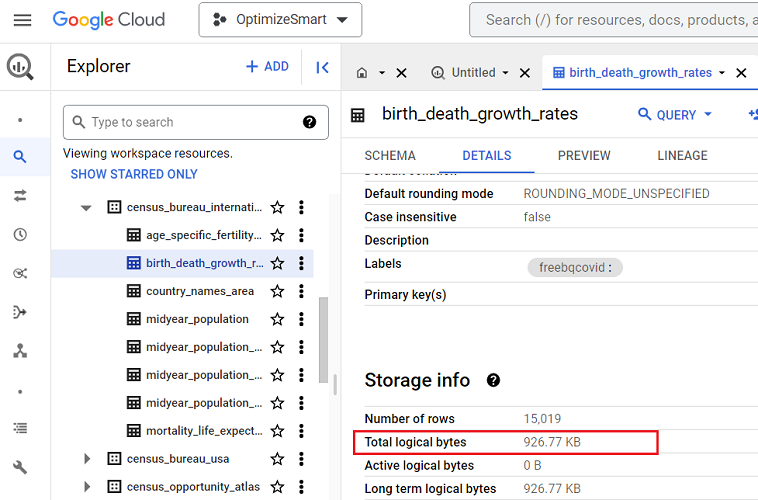
If the size of the data table is just a few kilobytes (KB) or megabytes (MB), you don’t need to worry.
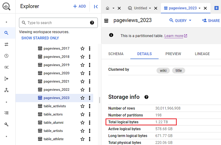
But if the table size is in gigabytes (GB), terabytes (TB) or petabytes (PB), you should be careful how you query your data.
For example, you should be careful when querying the following data table as it is in terabytes:
#4 Before you query the data from a table, preview the table.
Many people, especially new users, run queries just to preview the data in a data table.
This could considerably cost you if you accidentally queried gigabytes or terabytes of data.
Instead of running queries just to preview the data in a data table, click on the ‘Preview’ tab to preview the table.
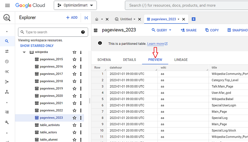
There is no cost for previewing the data table.
The table preview will give you an idea of what type of data is available in the table without querying the table.
#5 Always look at how much data your query will process before you run your query.
If your query is going to process only kilobytes or megabytes of data, then you don’t need to worry.
However, if your query is going to process gigabytes or terabytes of data, it could cost you considerably:
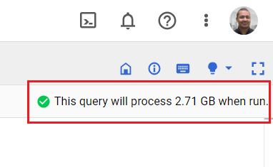
If that’s the case, query only that data, which is absolutely necessary.
#6 Your query cost depends on the number and/or size of the returned columns, not the rows.
Returning 10 rows/records is going to cost you the same as returning 10,000 records of data:
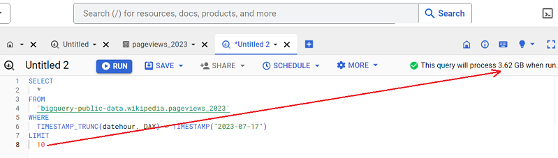
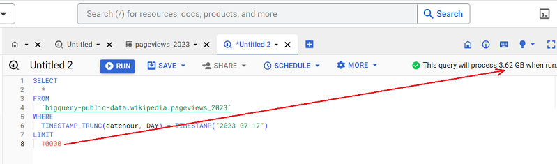
The number of rows/records your query returns does not affect your query cost.
Your query cost is affected by the number of columns your query returns.
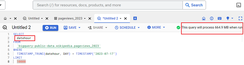
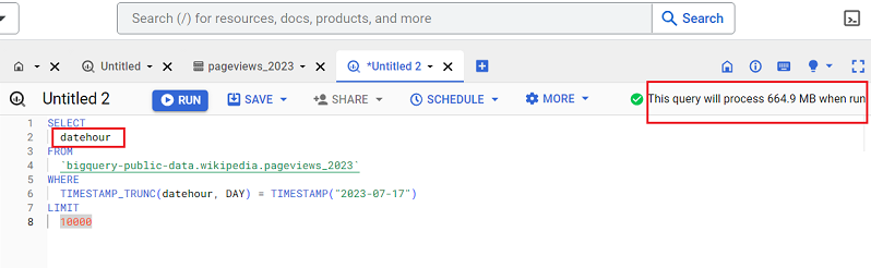
Following is an example of a query which would return one column named ‘datehour’:
Following is an example of a query which would return two columns named ‘datehour’ and ‘title’:
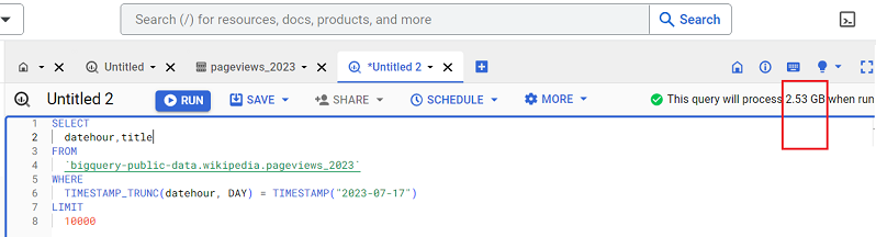
You can see from the screenshot how adding another column to the query increased the query size from 664.9 MB to a whopping 2.53 GB.
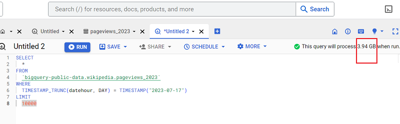
What would happen if we wrote a query that returns all the table columns?
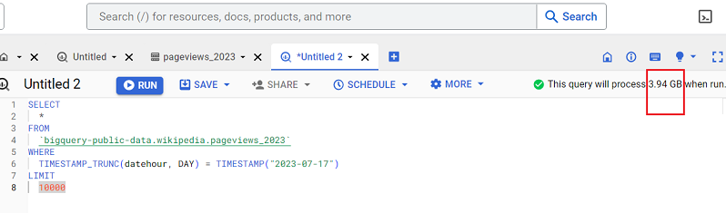
So if we try to return all the columns of this data table, 3.94 GB of the data would be processed.
So only query the columns you really need.
#7 Your query cost is also affected by the size of each column.
The query below returns one column named ‘datehour’:
The query below returns one column named ‘title’:
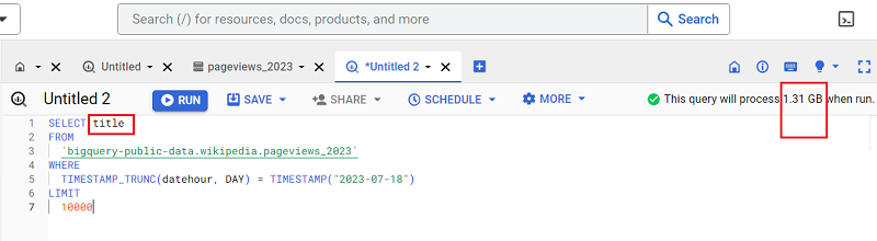
Note how the size of the query increased from 664.9 MB to 1.31 GB.
So you must be very careful about the size of the column you want to retrieve.
#8 Avoid using SELECT *
SELECT * means returns all the columns of the data table.
Now, if your data table contains a lot of columns and some of the columns are very big in size (maybe in GB or TB), using SELECT * could considerably increase your query cost.
So the best practice is to avoid using SELECT *
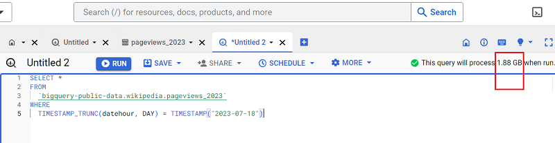
#9 Applying a LIMIT clause to a SELECT * query does not affect the query cost.
This is because the LIMIT clause controls the number of rows/records your query returns.
But as you know by now, the number of rows/records your query returns doesn’t affect your query cost.
With the LIMIT clause:
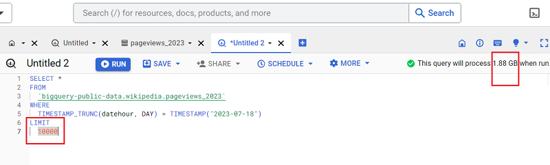
Without the LIMIT clause:
#10 Set up Budget alerts.
Set up cloud billing budgets and budget alerts which trigger email notifications to billing admins and/or project managers when your costs (actual costs or forecasted costs) exceed a percentage of your budget (based on the threshold rules you set).
These email alerts inform you of your usage costs trending over time.
Note: Setting up a budget does not automatically cap Google Cloud usage or spending.
For more information on setting up cloud billing budgets and budget alerts, check out the official help documentation from Google: https://cloud.google.com/billing/docs/how-to/budgets
#11 Set up Quota limits.
You can turn on cost control at a project level or user level by setting up/customizing quota limits.
That way, you can cap the maximum number of bytes processed per day by a given user or project.
When the user/project exceeds their quota limit, the query will not be processed, and a “quota exceeded” error message will be displayed.
To learn more about working with Quotas, check out the official help documentation from Google: https://cloud.google.com/docs/quota
#12 Regularly monitor your spending.
At least once a week, visit the ‘Billing‘ section of your Google Cloud Platform account to see how much you have spent so far:

#13 Use the Google Cloud Pricing Calculator.
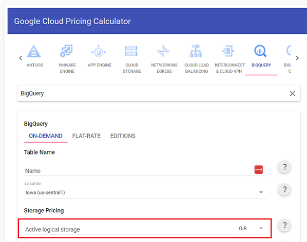
The Google Cloud pricing calculator estimates the monthly storage cost and/or cost of running your desired queries before you actually run them.
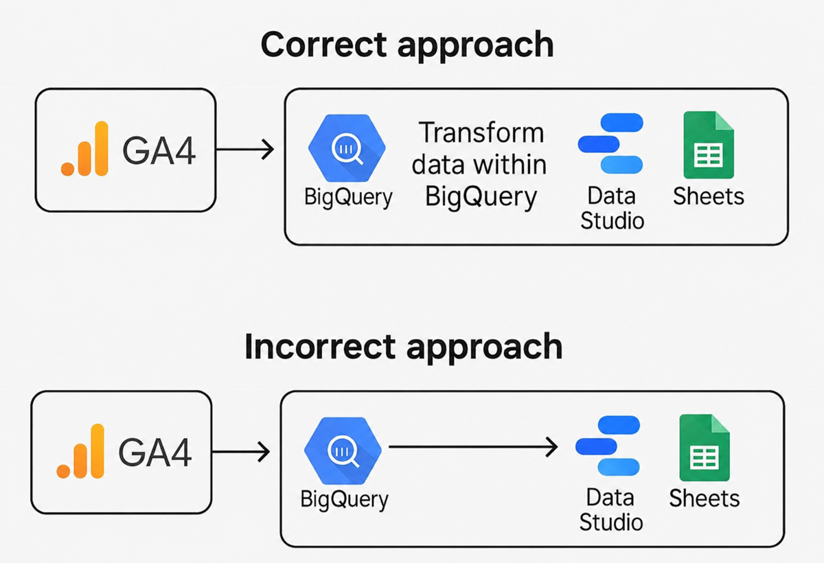
#14 Transform BigQuery data before you send it to data platforms (like Data Studio or Google Sheets).
For ongoing or production dashboards, avoid connecting reporting tools (like Data Studio or Google Sheets) directly to raw BigQuery tables, especially once your tables are larger than a few GB or your reports are used regularly.
This simple change can save you thousands in data processing costs each month.
Many BigQuery users connect destination data platforms (such as Google Sheets or Data Studio) directly to raw BigQuery tables without first transforming the data.
This leads to:
>> Every interaction with the data platform can re‑run a query like SELECT * FROM raw_table or FROM events_* with no date filter, causing BigQuery to scan the entire table or full history each time.
>> All columns and rows are being processed, even if only a subset is needed.
>> Massive, unnecessary data processing costs, especially with large tables.
Suppose you connected your Data Studio report directly to your BigQuery raw data table.
Now, every interaction with your report could result in you querying the entire raw data table in BigQuery.
If the raw data table is in GB or TB, you could end up querying GB/TB of data just by interacting with a Data Studio report for a couple of minutes.
Why does this happen?
>> Data platforms don't know which columns you need, so they fetch everything.
>> Raw tables often contain many columns and rows that are irrelevant for reporting.
>> BigQuery charges based on the amount of data processed, not just the number of queries.
The fix is to build a reporting layer inside BigQuery.
Before extracting data from BigQuery, you should transform and prepare it within BigQuery, which involves removing unnecessary columns and rows and formatting it in a way that the destination data platform can understand.
You may also need to partition the data, which will help reduce the amount of data needed for each query.
Instead of extracting data directly from raw data tables, extract data from partitioned tables.
Instead of connecting your destination data platforms directly to raw data tables in BigQuery, connect to partitioned tables.
GA4 BigQuery data is already partitioned by dates.
However, that may still not be enough (depending on your website traffic), and you may need to perform further partitioning, such as row-based partitioning or expression-based partitioning, to reduce the size of your queries and the data processing cost.
How to build the reporting layer?
Start with plain BigQuery SQL and scheduled queries if your reporting layer is small.
>> Write SQL to transform raw tables (for example GA4 events_*) into lean reporting tables or views with only the columns and date ranges you need.
>> Use BigQuery features like partitioning, clustering, and scheduled queries to keep scans small and updates automated without additional tooling.
As your setup grows (more tables, more clients or properties, multiple environments, and logic that changes over time), introduce a transformation framework such as Dataform, dbt, or SQLMesh:
>> These tools manage SQL‑based pipelines in BigQuery with dependency graphs, automated builds, and orchestration.
>> They add testing, documentation, version control, environments, and lineage, letting you evolve your reporting layer safely as dashboards and business requirements expand.
If you’re staying 100% on BigQuery, Dataform is the best default choice, with dbt as a strong alternative if you want ecosystem portability or already think in dbt terms. SQLMesh becomes more niche.
Dataform is designed specifically for SQL pipelines on BigQuery. It runs natively in BigQuery/BigQuery Studio; no separate infra to manage.
Think of it as ETL, not just export.
Extract: Pull raw data (e.g., GA4 BigQuery export).
Transform: Before loading the data elsewhere, transform it within BigQuery. Clean, filter, and format data; remove unnecessary columns/rows; partition data for efficiency.
Load: Once the data has been transformed and partitioned, load it into your destination data platform (e.g., Looker, Google Sheets).
Factors which determine BigQuery Cost for your company.
Your monthly cost of using BigQuery depends upon the following factors (but is not limited to):
#1 The amount of data you store in BigQuery (i.e. the data storage cost)
#2 The amount of data you processed by each query you run (i.e. the data processing cost).
#3 The amount of data you transfer in and out of BigQuery (i.e. the data transfer cost).
#4 The cost associated with the type of BigQuery Edition (‘Standard’, ‘Enterprise’, ‘Dedicated’) you use (i.e. the BigQuery edition cost).
The initial 10 GB of active storage each month is free. Beyond that, you will incur a fee of $0.020 per GB for active storage.
Each month, the first 1 terabyte of processed data is also included in the free tier. Any additional processed data will be billed at $5 per terabyte (TB).
As long as you stay within the 10 GB storage limit and the 1 terabyte query limit per month, there will be no charges to your credit card.
Your credit card will be charged only when you exceed these free limits.
Suppose you begin querying terabytes or petabytes of data daily in BigQuery. In that case, be prepared for substantial monthly data storage and/or data processing fees.
BigQuery operations that are free of charge.
The following BigQuery operations are free of charge in any location:
- The first 10 GiB per month of storage is free.
- The first 1 TB of query data processed per month is free.
- Queries that result in an error are free of charge.
- Cached queries.
- Deleting tables, views, partitions, functions and datasets
For more details, refer to the official BigQuery pricing documentation.
Related Article: BigQuery Storage Explained.
Related Articles:
- Tracking Pages With No Traffic in GA4 BigQuery.
- First User Primary Channel Group in GA4 BigQuery
- How to handle empty fields in GA4 BigQuery.
- Extracting GA4 User Properties in BigQuery.
- Calculating New vs Returning GA4 Users in BigQuery.
- How to access BigQuery Public Data Sets.
- How to access GA4 Sample Data in BigQuery.
- Understanding engagement_time_msec in GA4 BigQuery.
- GA4 BigQuery Attribution Tutorial.
- How to backfill GA4 data in BigQuery.
- How to send data from Google Search Console to BigQuery.
- Google Advanced Consent Mode and GA4 BigQuery Export.
- Google Analytics 4 BigQuery Tutorial for Beginners to Advanced.
- Prompt Engineering for GA4 BigQuery SQL Generation.
- How to create a new BigQuery project.
- How to create a new Google Cloud Platform account.
- How to overcome GA4 BigQuery Export limit.
- BigQuery Cost Optimization Best Practices.
- event_timestamp vs user_first_touch_timestamp GA4 BigQuery.
- GA4 BigQuery Video Tracking Report.